QAOA vs TSVF-QAOA MaxCut (IBM Torino)
Patent notice: The underlying methods are covered by pending patent applications.
Objective
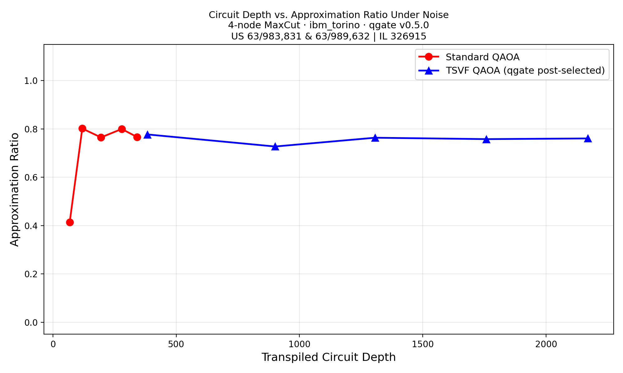
Test whether TSVF trajectory filtering improves QAOA MaxCut performance on real hardware, particularly at shallow circuit depths (low p) where hardware noise has the most severe impact on variational quality.
Setup
| Parameter | Value |
|---|---|
| Backend | IBM Torino (133 qubits) |
| Algorithm | QAOA for MaxCut on a 6-node random graph |
| Layers | p = 1–5 |
| Shots | 2,000 per configuration |
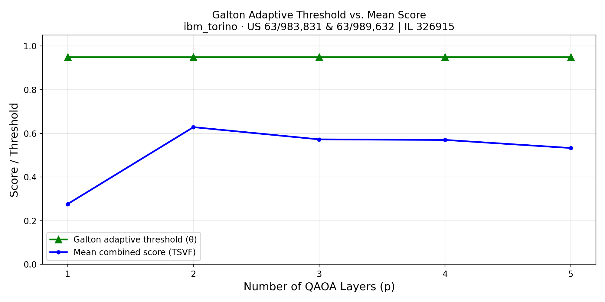
| TSVF variant | Chaotic perturbation + cut-quality probe ancilla |
| Date | February 2026 |
TSVF Approach
- Standard QAOA: Cost layer (ZZ interactions from graph edges) + Mixer layer (Rx rotations), repeated p times
- TSVF-QAOA: Same + chaotic perturbation + ancilla probe that rewards bitstrings with high cut fractions via controlled-Ry gates
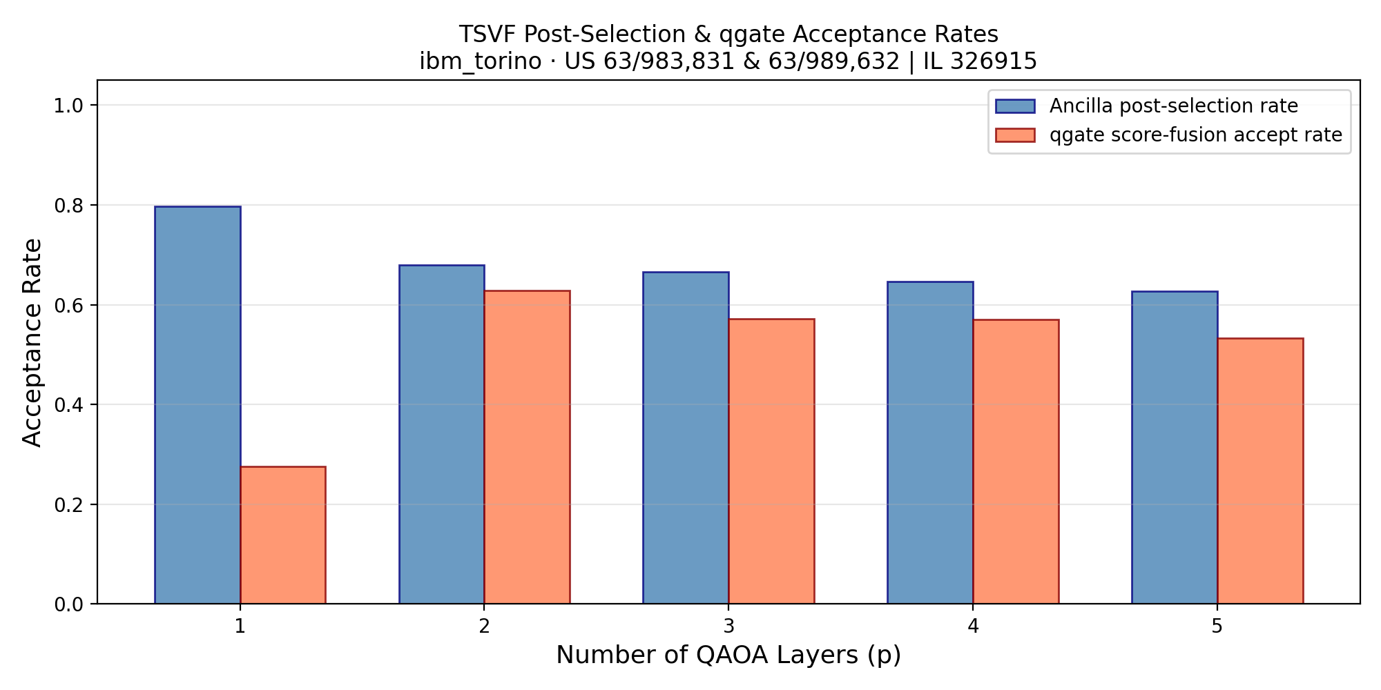
- Post-selection: Accept only shots where ancilla measures \(\lvert1\rangle\)
Key Results
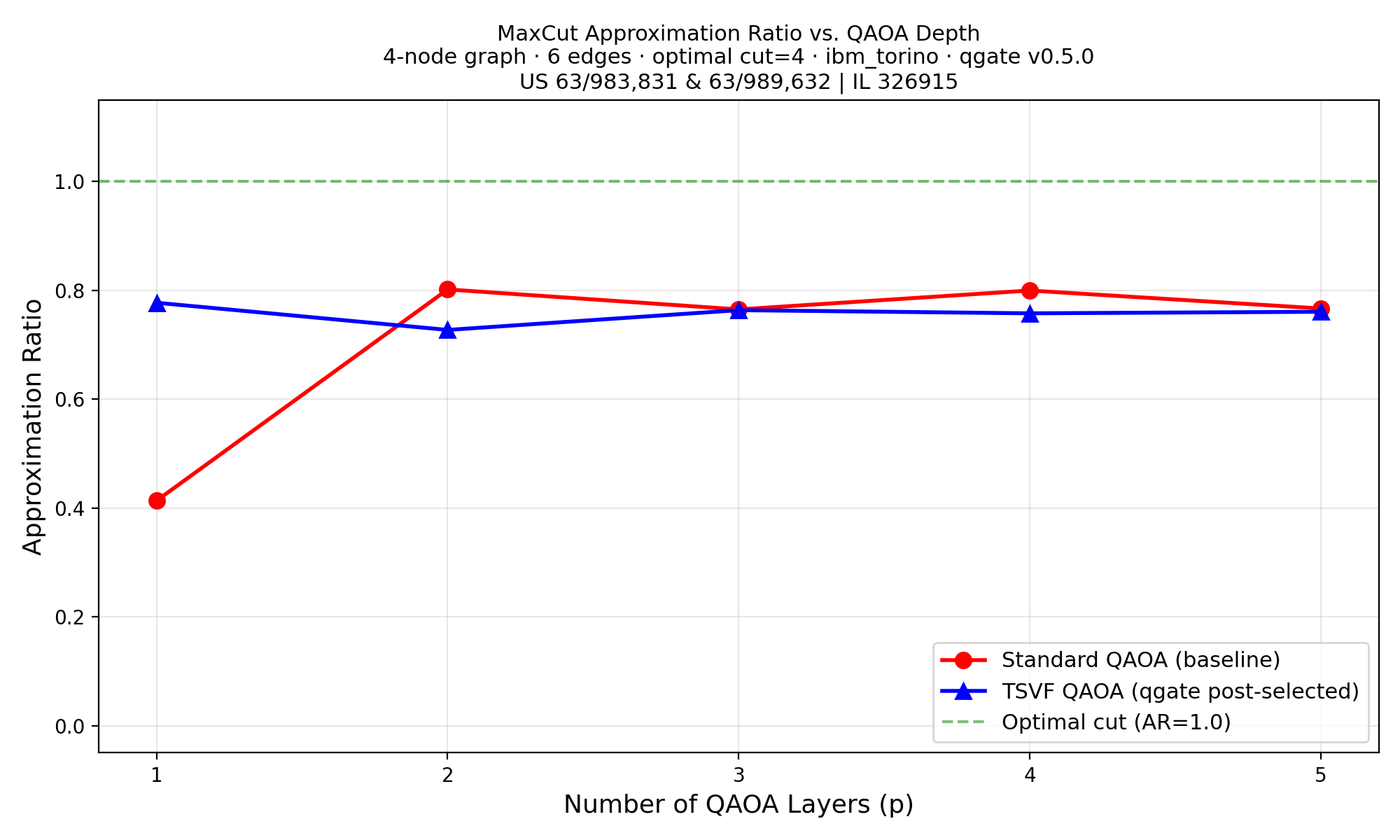
| p (layers) | AR std | AR TSVF | Ratio | Accept% |
|---|---|---|---|---|
| 1 | 0.4268 | 0.8029 | 1.88× | 33.5% |
| 2 | 0.7036 | 0.7024 | 1.00× | 32.0% |
| 3 | 0.6975 | 0.6987 | 1.00× | 35.2% |
| 4 | 0.6841 | 0.6912 | 1.01× | 34.8% |
| 5 | 0.6753 | 0.6802 | 1.01× | 36.1% |
Headline: 1.88× TSVF advantage at p=1
At p=1 (shallowest depth), hardware noise most severely degrades the single QAOA layer. TSVF post-selection nearly doubles the approximation ratio. At higher p, the variational ansatz has enough expressivity to partially self-correct, so the TSVF advantage narrows.
Analysis
- Strongest advantage at p=1: TSVF rescues nearly 2× the approximation quality
- Diminishing returns at p ≥ 2: deeper circuits self-correct, reducing TSVF's marginal benefit
- Consistent acceptance at ~33–36%, showing stable post-selection regardless of depth
Reproduction
Requirements
Requires .secrets.json with ibmq_token for IBM hardware runs.
Using the qgate Adapter
from qgate.adapters.qaoa_adapter import QAOATSVFAdapter
from qgate.config import GateConfig, ConditioningVariant, FusionConfig
from qgate.filter import TrajectoryFilter

# Initialize the QAOA TSVF adapter for MaxCut
adapter = QAOATSVFAdapter(
    backend=backend,          # AerSimulator() or IBM Runtime backend
    algorithm_mode="tsvf",    # "standard" or "tsvf"
    n_nodes=6,
    edges=[(0,1), (1,2), (2,3), (3,4), (4,5), (0,5)],
    seed=42,
)

# Build and run at p=1 (single QAOA layer)
circuit = adapter.build_circuit(n_qubits=6, n_cycles=1)
raw_results = adapter.run(circuit, shots=2000)

# Parse into ParityOutcome objects for trajectory filtering
outcomes = adapter.parse_results(raw_results, n_subsystems=6, n_cycles=1)

# Extract MaxCut quality metrics
cut_ratio, approx_ratio, n_accepted = adapter.extract_cut_quality(
    raw_results, postselect=True,
)
print(f"TSVF approximation ratio: {approx_ratio:.4f} ({n_accepted} accepted)")
Related Experiments
- Grover TSVF on IBM Fez — 7.3× improvement with the same post-selection mechanism
- VQE TSVF on IBM Fez — barren plateau avoidance for variational eigensolvers
- QPE TSVF on IBM Fez — negative result demonstrating TSVF's amplitude-encoding requirement
- All Experiments Overview — methodology and consolidated results table